Introduction: The Game of Life
You can hardly find a programmer who heard about Conway’s Game of Life but has never tried to program it. Google programmers are no exception, otherwise they wouldn’t have included a Life interpreter into the respective search result page. I am no exception either. The first time I tried to do it was on one ancient computer, which you are unlikely to see even in a museum these days. The processor was so slow and the field was so small that I didn’t even bother to measure performance. Next time it was on an 8-bit 1 MHz processor. If I remember correctly, an assembly program could process 256×256 matrix in 6s. It seemed fast in those days. Since the algorithm was matrix-based (the program worked right inside the video memory), half the size meant four times the speed. A 32×32 matrix produced a movie with 10 fps. I haven’t tried it on modern machines and/or in Java yet, so I got curious: what speed is achievable now? The clock frequency has become 2,500 times higher since then. If the speed keeps up with the CPU clock, we should be able to process 256×256 at 400 fps. But our processor is 64-bit, so in theory it could do 3200 fps. Is it possible?
The rules
The Life universe is an infinite two-dimensional square grid with some squares occupied by live cells. Each square has eight neighbours, direct and diagonal. The game time runs in clock ticks, and on each tick, the following events happen:
- The number of live neighbours is calculated for each square
- All the cells having less than two live neighbours die of solitude
- All the cells having more than three live neighbours die of overpopulation
- A new cell is born on each empty square that has three live neighbours.
The game received attention from researchers, and many interesting structures have been found: stable static structures, oscillators, moving patterns (gliders), and lots of more complex objects. Certain initial patterns, albeit small, evolve for quite a while and produce non-trivial results. Here is an example: this simple structure (R-pentamino piece) starts small, grows, lives a turbulent life and then deteriorates and fades away, never dying completely:
You can click “Start” and see how this one evolves.
What about hash tables?
But wait, this article must have something to do with hash tables and hash codes. In which way are they relevant to Life?
There are two major classes of Life programs. The matrix-based ones, such as those in my old experiments, store a part of the universe (or the entire universe considered being a toroidal array, as in the examples above) as a matrix. The entire matrix is re-calculated on each step. These programs are very simple but have two disadvantages. Firstly, they are limited by the size of the matrix, and Life structures are known to be able to grow indefinitely (for example, by spawning gliders). This means such programs can only produce approximate results, such as the result we saw for the R-pentamino above. Secondly, most Life colonies contain much fewer live cells than there’re squares in the matrix, which suggests a way of improving speed – to keep track of the occupied cells in some data structure and only process those. This is the second class of Life programs. Very sophisticated data structures have been used for Life simulation, some with extraordinary performance. For instance, the HashLife approach makes use of identifying repeating patterns both in space and time, with great results.
I want to do something much simpler than HashLife – use a data structure that is readily available in Java – the HashMap
(and its buddy HashSet). This has an additional advantage that the HashMap is used a lot in production
Java code, so learning something about it may prove useful in general programming practice.
The timing results, however, won’t be directly comparable with my old results, since the algorithms are different. I’ll try the matrix approach later too.
The test
It is not trivial to find a suitable test input for a Life program. An arbitrary set of cells is very likely to die very quickly. We’ve seen one simple structure that lived for a while, the R-pentamino. Here is another one, the acorn:
We’ll be using the acorn as it lives a bit longer, and grows bigger – it stabilises at 633 living cells while the R-pentamino does at 116.
The plan
The algorithm is very simple, and the initial implementation will be based directly on the classes provided by Java library.
We’ll represent locations on the grid as values of class Point, encapsulating two co-ordinates, x and y.
This class will be equipped with appropriate equals() and hashCode() methods to be used as a hash map key.
Then we can maintain a state of the colony (which we’ll call “field”) simply as a set of Point objects (HashSet will do). We’ll use int values as our
co-ordinates, allowing both positive and negative ones. This means that the grid is still finite and will wrap around at some
point, so simulations of unbounded structures, such as gliders, will be limited in time (although I’d be very happy
if I could hit this limitation in real life – that would mean that the program performed several billion iterations in
reasonable time, and this is something yet to be achieved). Another consideration
is memory. There are configurations that grow indefinitely, such as Gosper Glider Gun:
If we simulate this gun long enough, we’ll run out of memory. However, a million or two iterations should still work. Perhaps, we’ll do the gun next time.
The code
The code can be found here.
First of all, we need a Point class. Here it is:
class Point
{
    public final int x, y;

    public Point (int x, int y)
    {
        this.x = x;
        this.y = y;
    }

    @Override
    public final boolean equals (Object obj)
    {
        Point p = (Point) obj;
        return x == p.x && y == p.y;
    }

    @Override
    public final int hashCode ()
    {
        return x * 3 + y * 5;
    }

    @Override
    public String toString ()
    {
        return "(" + x + "," + y + ")";
    }

    public Point[] neighbours ()
    {
        return new Point[] {
            new Point (x-1, y-1),
            new Point (x-1, y),
            new Point (x-1, y+1),
            new Point (x, y-1),
            new Point (x, y+1),
            new Point (x+1, y-1),
            new Point (x+1, y),
            new Point (x+1, y+1)
        };
    }
}
The only part of this class worth explanation is the hashCode() method. Why such hash function?
We need something that depends on both numbers in a not-completely-trivial way. Multiplying
by some prime numbers and adding the results seems good enough. We’ll come back to this issue later.
We’ll use a HashSet of Points as a field:
public static final int HASH_SIZE = 8192;
private HashSet<Point> field = new HashSet<Point> (HASH_SIZE);
Specifying an initial size (8192) avoids spending time growing the table. This isn’t very important, it just simplifies performance comparisons.
We’ll also maintain another structure, counts:
private HashMap<Point, Integer> counts =
        new HashMap<Point, Integer> (HASH_SIZE);
It will contain the number of live neighbours for each square. Zero will be assumed for squares not included in this map; the reverse will be maintained in the first implementation – a square will be removed from the map when its neighbour count becomes zero. This isn’t necessarily the best strategy – we may reconsider it later.
We’ll update this structure each time we create or destroy a living cell:
private void inc (Point w)
{
    Integer c = counts.get (w);
    counts.put (w, c == null ? 1 : c + 1);
}

private void dec (Point w)
{
    int c = counts.get (w) - 1;
    if (c != 0) {
        counts.put (w, c);
    } else {
        counts.remove (w);
    }
}

void set (Point w)
{
    for (Point p : w.neighbours ()) {
        inc (p);
    }
    field.add (w);
}

void reset (Point w)
{
    for (Point p : w.neighbours ()) {
        dec (p);
    }
    field.remove (w);
}
We can immediately see some inefficiencies in the code. For instance, set() calls neighbours(), which allocates
an array and eight Point objects. We can’t avoid creating these Point objects (we need something as hash map keys),
but could do without array creation. Another example is the counts hash map. Code like
int c = counts.get (w) - 1;
counts.put (w, c);
gives an impression that the map holds primitive values of type int, which are updated when we call put().
This illusion is a result of Java’s automatic boxing. Actually, the map contains objects of the class Integer,
and a new object is allocated each time a value changes. This is hardly the most efficient way to store numbers in a hash table.
But we’ll ignore these inefficiencies for now. Let’s first see what speed we can achieve without any optimisations.
Still missing is the main step operation:
public void step ()
{
    ArrayList<Point> toReset = new ArrayList<Point> ();
    ArrayList<Point> toSet = new ArrayList<Point> ();
    for (Point w : field) {
        Integer c = counts.get (w);
        if (c == null || c < 2 || c > 3) toReset.add (w);
    }
    for (Point w : counts.keySet ()) {
        if (counts.get (w) == 3 && ! field.contains (w)) toSet.add (w);
    }
    for (Point w : toReset) {
        reset (w);
    }
    for (Point w : toSet) {
        set (w);
    }
}
Methods set() and reset() modify both field and counts, so we can’t call them inside two main loops. We have
to memorise the cells that must be created and destroyed and perform the operations later. The reset() pass
is performed before set() in the hope to make it a little bit faster (hash table operations run faster when there are
fewer elements in the table).
There is also usual correctness check code, which isn’t needed now but will be important later, and the performance measurement code. We’ll run each performance test three times. Here is the run result:
# java -server Life
  Hash_Reference: time for 10000:  2937  2719  2763: 3619.3 frames/sec
How good is it? Interestingly, it is of the same order of magnitude as the 3,200 fps I was talking about in the beginning of the article. However, the algorithms are of different nature, so the results aren’t directly comparable.
Going Long
A very obvious optimisation comes to mind when one looks at this code: getting rid of the Point class. Why store two
32-bit values separately if they can be packed into one 64-bit long value? This looks especially attractive on a 64-bit
platform. We can immediately see two
advantages: we don’t need a special class (the built-in long type is sufficient), and we use only one CPU instruction
comparing the values instead of two (three, if you count a branch). There is also another, not so obvious
advantage: we can enumerate neighbouring positions for a square by adding eight statically known offsets to the corresponding long.
There is a disadvantage, too: the code loses some clarity and type safety. A Point is much more informative than
a long. You can’t by mistake pass a loop index or current time as a Point, but you can as a long. A Point
gives immediate access to its components (x and y), while long must still be decoded, and it is much easier
to make a mistake there. In short, if we get a speed increase, it will come with a price tag. This is a common case with optimisation.
There are some interesting technical details, too. Here is the code we use to combine two int values into one long
and split it back:
public static long w (int hi, int lo)
{
    return ((long) hi << 32) | lo & 0xFFFFFFFFL;
}

public static int hi (long w)
{
    return (int) (w >>> 32);
}

public static int lo (long w)
{
    return (int) w;
}
The significance of & 0xFFFFFFFFL (and of that trailing L) is known to every experienced Java programmer,
because few of them haven’t made a mistake in such code at least once. When converted to long, int values are
sign-extended. As a result, the entire high part of a w() result would be filled with ones for any negative lo
unless it is first converted to a long and then ANDed with the appropriate mask.
Storing x and y together in a long makes it easy to calculate positions of the neighbours.
Here is what the set() method looks like using longs:
public static final long DX = 0x100000000L;
public static final long DY = 1;

void set (long w)
{
    inc (w-DX-DY);
    inc (w-DX);
    inc (w-DX+DY);
    inc (w-DY);
    inc (w+DY);
    inc (w+DX-DY);
    inc (w+DX);
    inc (w+DX+DY);
    field.add (w);
}
These formulas, however, do not tolerate transitions across zero. For instance, a formula for the top left
neighbour is w-DX-DY. For location (1, 1) it gives correct result (0, 0), but for (0, 0) it produces
which is (-2, -1) instead of (-1, -1). To resolve this, we’ll add
an offset of 0x80000000 to all co-ordinates. This offset is only applied at input and output time, and does not
affect the main algorithm:
public static final int offset = 0x80000000;

public static int x (long w)
{
    return hi (w) - OFFSET;
}

public static int y (long w)
{
    return lo (w) - OFFSET;
}

public static long fromPoint (int x, int y)
{
    return w (x + OFFSET, y + OFFSET);
}
The rest of the program stays virtually unchanged. We’ll run the test alone – comment out the test for Point in main () and leave only
the new one. This will remove any possible effects one test can have on another. Here is the result:
# java -server Life
       Hash_Long: time for 10000:  4290  4237  4273: 2340.3 frames/sec
What a surprise! The performance got worse. What went wrong? It seems very unlikely that operations with long,
even boxed as Long, are slower than with our Point class. The general structure of the program is the same. What is the difference?
The difference is in the hashCode() method. In the Point class it looked like this:
public final int hashCode ()
{
    return x * 3 + y * 5;
}
And here is the same method from the standard class Long:
public int hashCode() {
    return (int)(value ^ (value >>> 32));
}
Can this be the reason?
Could the difference in hash functions have caused such performance difference? This is easy to check. We’ll write
a version similar to the one based on long but with the same hash code as the original one. Extending the Long
class would have done the trick, but this is impossible, because that class is final (besides, boxing would have created values of
the original class anyway). We need to write our own version of Long, with modified hash code. Obviously,
automatic boxing and unboxing will not happen. In fact, this class has very little in common with Long,
so it’s better to call it a different version of Point:
final class LongPoint extends LongUtil
{
    final long v;

    public LongPoint (long v)
    {
        this.v = v;
    }

    public LongPoint (int x, int y)
    {
        this.v = fromPoint (x, y);
    }

    public Point toPoint ()
    {
        return toPoint (v);
    }

    @Override
    public boolean equals (Object v2)
    {
        return ((LongPoint) v2).v == v;
    }

    @Override
    public int hashCode ()
    {
        return hi(v) * 3 + lo(v) * 5;
    }

    @Override
    public String toString ()
    {
        return toPoint().toString ();
    }
}
A pedantic reader would point out that this class isn’t equivalent to the original version, since its hashCode() uses x and y
values with added OFFSET. However, this won’t affect either the time to compute the hash or the quality of hashing. In
fact, the hash value will be exactly the same: 0x80000000 multiplied by 3 (or 5) as int is still 0x80000000,
and the two added together will cancel each other out.
Since there is no more boxing, the code is a little bit longer, but it is also clearer and safer – arbitrary number can’t be passed as a point anymore. Again, I’ll run it alone. Here is the result (I’ll quote all three):
  Hash_Reference: time for 10000:  2937  2719  2763: 3619.3 frames/sec
       Hash_Long: time for 10000:  4290  4237  4273: 2340.3 frames/sec
  Hash_LongPoint: time for 10000:  2864  2651  2602: 3843.2 frames/sec
This proves our theory. The version using long with the hash formula from Point is much faster than the one with
the built-in hash function of Long. It is also a bit faster than the original Point-based version, which proves
that there is indeed some advantage in packing numbers in long.
How good are your hash codes?
At last, we arrived at the main topic of the article: the hash codes. Very few programmers fine-tune their hash functions, relying either on default implementations, or on those that intuitively seem good. But, as we have just seen, the choice of a hash function has significant impact on performance (50% slowdown in our case). Why?
Java uses a classic hash map structure, which features an array of a certain “big enough” size and a direct mapping
of hash codes to positions in this array, called slots. Typically the hash value is divided by the array size and the remainder is
used as an index. This is how the HashTable was implemented. In HashMap, the array size is always a power of two,
so the remainder operation is replaced with a bitwise AND – the required number of lowest bits is taken.
It would be great to develop a hash function, which, provided that the number of entries is less than the array size,
would map them all to different slots. Perhaps, this can be achieved in some special cases, but not in a general-purpose
implementation. This means that such implementation must deal with hash collisions. A classic hash map
does that by storing more than one entry per slot in some data collection, most commonly a linked list.
This is what Java 7 does. Java 8 introduces
a change: it uses binary trees for long chains (eight elements and more).
We’ll concentrate on Java 7 for now (most of findings are also applicable to Java 8, since chains of eight and more
elements are a pathological case).
Each insert operation requires a traversal of the entire list for the given slot,
and so does each unsuccessful lookup. An average successful
lookup requires a traversal of half the list. In short, the number of inspected entries is roughly
proportional to the average length of the list, which equals the number of elements in the hash table
divided by the number of non-empty slots. So we need the hash function to spread values evenly across the array.
Probably, both the above hash functions would work well if x and y values were truly random 32-bit numbers.
However, our co-ordinates, as most real life values, are not random; they follow some patterns, and hash functions
may react badly to those patterns. This means that some hash functions may be much better than the other ones for
specific tasks, one example of which we have just seen.
The full hash value is kept in each hash map entry. When traversing a chain, the hash map implementation checks it first,
only calling equals() on objects if their hashes are equal. As a result, a full hash collision (where two hash values are equal)
is worse than a partial collision (where two hashes are different but still fall into the same slot), although both
reduce performance.
Java 7 employs the following technique to reduce the number of partial collisions. The HashMap does not directly use the lowest bits of a hash code. It first applies
some additional bit manipulations:
final int hash(Object k) {
    int h = hashSeed;
    if (0 != h && k instanceof String) {
        return sun.misc.Hashing.stringHash32((String) k);
    }

    h ^= k.hashCode();

    // This function ensures that hashCodes that differ only by
    // constant multiples at each bit position have a bounded
    // number of collisions (approximately 8 at default load factor).
    h ^= (h >>> 20) ^ (h >>> 12);
    return h ^ (h >>> 7) ^ (h >>> 4);
}
This bit shuffling helps against hash functions that generate a sufficient number of different values, but
those values differ mostly in higher-order bits and therefore hit a small number of slots.
This shuffling has been removed in Java 8 – binary trees are supposed to
take care of partial conflicts. However, neither bit shuffling nor binary trees help against full hash conflicts, which originate
from poor-quality hash functions that generate too few distinct hash values for the given set of inputs.
And the XOR-based hash code of Long is exactly like that. For instance, it maps the entire
diagonal line (0,0), (1,1), (2,2), … into the single value 0:
| x | |||||||||||||||||
|---|---|---|---|---|---|---|---|---|---|---|---|---|---|---|---|---|---|
| 0 | 1 | 2 | 3 | 4 | 5 | 6 | 7 | 8 | 9 | 10 | 11 | 12 | 13 | 14 | 15 | ||
| y | |||||||||||||||||
| 0 | 0 | 1 | 2 | 3 | 4 | 5 | 6 | 7 | 8 | 9 | 10 | 11 | 12 | 13 | 14 | 15 | |
| 1 | 1 | 0 | 3 | 2 | 5 | 4 | 7 | 6 | 9 | 8 | 11 | 10 | 13 | 12 | 15 | 14 | |
| 2 | 2 | 3 | 0 | 1 | 6 | 7 | 4 | 5 | 10 | 11 | 8 | 9 | 14 | 15 | 12 | 13 | |
| 3 | 3 | 2 | 1 | 0 | 7 | 6 | 5 | 4 | 11 | 10 | 9 | 8 | 15 | 14 | 13 | 12 | |
| 4 | 4 | 5 | 6 | 7 | 0 | 1 | 2 | 3 | 12 | 13 | 14 | 15 | 8 | 9 | 10 | 11 | |
| 5 | 5 | 4 | 7 | 6 | 1 | 0 | 3 | 2 | 13 | 12 | 15 | 14 | 9 | 8 | 11 | 10 | |
| 6 | 6 | 7 | 4 | 5 | 2 | 3 | 0 | 1 | 14 | 15 | 12 | 13 | 10 | 11 | 8 | 9 | |
| 7 | 7 | 6 | 5 | 4 | 3 | 2 | 1 | 0 | 15 | 14 | 13 | 12 | 11 | 10 | 9 | 8 | |
| 8 | 8 | 9 | 10 | 11 | 12 | 13 | 14 | 15 | 0 | 1 | 2 | 3 | 4 | 5 | 6 | 7 | |
| 9 | 9 | 8 | 11 | 10 | 13 | 12 | 15 | 14 | 1 | 0 | 3 | 2 | 5 | 4 | 7 | 6 | |
| 10 | 10 | 11 | 8 | 9 | 14 | 15 | 12 | 13 | 2 | 3 | 0 | 1 | 6 | 7 | 4 | 5 | |
| 11 | 11 | 10 | 9 | 8 | 15 | 14 | 13 | 12 | 3 | 2 | 1 | 0 | 7 | 6 | 5 | 4 | |
| 12 | 12 | 13 | 14 | 15 | 8 | 9 | 10 | 11 | 4 | 5 | 6 | 7 | 0 | 1 | 2 | 3 | |
| 13 | 13 | 12 | 15 | 14 | 9 | 8 | 11 | 10 | 5 | 4 | 7 | 6 | 1 | 0 | 3 | 2 | |
| 14 | 14 | 15 | 12 | 13 | 10 | 11 | 8 | 9 | 6 | 7 | 4 | 5 | 2 | 3 | 0 | 1 | |
| 15 | 15 | 14 | 13 | 12 | 11 | 10 | 9 | 8 | 7 | 6 | 5 | 4 | 3 | 2 | 1 | 0 | |
It does not work well with other diagonals, either.
Every other hash code for the diagonal y = x + 1 will be 1, every fourth – 3, and so on.
The codes for the diagonal y = x + 8 come in groups of eight identical values, and so on.
Patterns in a Life
game often contain diagonal lines or develop in a diagonal direction, so this behaviour is quite bad for performance.
The counts map suffers especially badly, since it contains both (x-1, y-1) and (x+1, y+1) keys for every live cell (x, y),
and that cell itself is very likely to feature as a key as well.
Our original hash
function (x * 3 + y * 5) behaves much better – it always maps a diagonal of size 100 into 100 different numbers.
The default hash function also behaves badly with patterns bounded by small squares. Consider a 32×32 square block,
where 0 ≤ x ≤ 31, 0 ≤ y ≤ 31. Each co-ordinate fits into 5 bits. A XOR of two co-ordinates also fits in 5 bits,
which means that the entire block (1,024 cells) is mapped to 32 hash codes. It can be a bit better for other blocks
(for instance, a 32×32 block positioned at (3, 38) maps to 100 values), but we want it to be as close to 1,024
as possible. Life colonies often fall apart into relatively small components, such as individual gliders or
pulsars, so this is important.
Our original hash function maps every 32×32 block into exactly 241 values, which is better, but still very far from optimal, which suggests that this function is not very good either. There are also cases where it fails miserably. For instance, it maps the entire line
y = (int) (x * -3.0/5.0) + y0;to just five values. This situation seems exotic, but we can’t trust our intuition here. We need a proper measurement to choose our hash function.
Measuring hash functions
We don’t have access to HashMap internals. The relevant fields and methods are package-private. The easiest is
to run our own simulation. We’ll start with printing the sizes and bounding rectangles as a function of time:
private static void sizeDump ()
{
    Hash_Reference r = new Hash_Reference ();
    put (r, ACORN);

    for (int i = 0; i < 10000; i++) {
        r.step ();
        int xmin = 0, xmax = 0, ymin = 0, ymax = 0;
        for (Point p : r.field) {
            xmin = Math.min (xmin,  p.x);
            xmax = Math.max (xmax,  p.x);
            ymin = Math.min (ymin,  p.y);
            ymax = Math.max (ymax,  p.y);
        }
        System.out.printf
            ("%5d: %5d - %5d; %5d - %5d; field size: %5d; counts size: %5d\n",
             i, xmin, xmax, ymin, ymax, r.field.size (), r.counts.size ());
    }
}
We had to modify Hash_Reference and made field and counts public.
As we can see, the colony grows at first, then shrinks a bit, and on step 5,205 stabilises at 633 living cells and 2,755 non-zero neighbours:
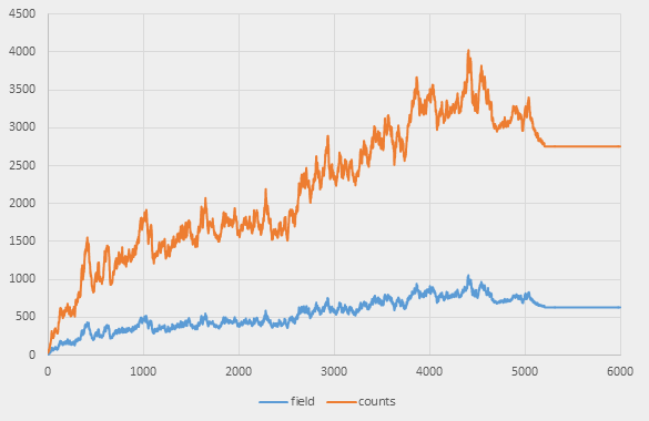
The maximum is reached roughly at step 4,400:
4400: -922 .. 1000; -1046 .. 1048; field size: 1034; counts size: 3938
It may seem that there is no point of running our test for 10,000 steps if the colony stalls long before that. Fortunately, it does not stall – the bounding rectangle keeps expanding:
9997: -2321 ..  2399; -2445 ..  2447; field size:   633; counts size:  2755
9998: -2321 ..  2400; -2445 ..  2447; field size:   633; counts size:  2755
9999: -2322 ..  2400; -2445 ..  2448; field size:   633; counts size:  2755
This is caused by some gliders flying away. A closer inspection of the colony shows that there are thirteen gliders and some pulsars. 108 cells die and 108 are born on each step – the test isn’t meaningless at all.
The best time to study the behaviour of hash tables is when they are fullest, so we’ll concentrate at step 4,400. Let’s apply various hash functions at this step and see how many slots in the 8,192-sized table are used:
private static int shuffle (int h)
{
    h ^= (h >>> 20) ^ (h >>> 12);
    h ^= (h >>> 7) ^ (h >>> 4);
    return h & (HASH_SIZE-1);
}

private interface Hash
{
    public int hash (Point p);
}

private static void hashtest (Hash h)
{
    Hash_Reference r = new Hash_Reference ();
    put (r, ACORN);

    int NSTEPS = 4400;

    for (int i = 0; i <= NSTEPS; i++) {
        r.step ();
    }

    BitSet b1 = new BitSet (HASH_SIZE);
    for (Point p : r.field) {
        b1.set (shuffle (h.hash (p)));
    }
    int nonzero_field = b1.cardinality ();
    double avg_field = (double) r.field.size () / nonzero_field;

    BitSet b2 = new BitSet (HASH_SIZE);
    for (Point p : r.counts.keySet ()) {
        b2.set (shuffle (h.hash (p)));
    }
    int nonzero_counts = b2.cardinality ();
    double avg_counts = (double) r.counts.size () / nonzero_counts;

    System.out.printf ("Field size: %4d; slots used: %4d; avg=%5.2f\n",
                       r.field.size (), nonzero_field, avg_field);
    System.out.printf ("Count size: %4d; slots used: %4d; avg=%5.2f\n",
                       r.counts.size (), nonzero_counts, avg_counts);
}
Now let’s try using it with different hashes:
First, the default hash for Long:
hashtest (new Hash () { public int hash (Point p) {
                          return p.x ^ p.y;}} );
This is where Lambda-definitions of Java 8 would be handy, but I’m testing it on Java 7.
Here is the result:
Field size: 1034; slots used:  240; avg= 4.31
Count size: 3938; slots used:  302; avg=13.04
The result really looks bad. List size of 13 is too big. With a table with the element count less than half the number of slots, we should be able to do better.
Now let’s look at our original Point hash:
hashtest (new Hash () { public int hash (Point p) {
                          return p.x * 3 + p.y * 5;}} );
Field size: 1034; slots used: 595; avg= 1.74
Count size: 3938; slots used: 1108; avg= 3.55
This is much better, so we’ve got the explanation of poor performance of Long compared to Point. However, in
absolute terms the result is still bad. Surely, we must be able to spread 3,938 entries across more
than 1,108 slots in a 8,192-sized hash table.
It looks like multiplying by 3 and 5 does not shuffle the bits well enough. How about some other prime numbers? Let’s try 11 and 17.
hashtest (new Hash () { public int hash (Point p) {
                          return p.x * 11 + p.y * 17;}} );
Field size: 1034; slots used: 885; avg= 1.17
Count size: 3938; slots used: 2252; avg= 1.75
That’s better. How about even bigger numbers?
hashtest (new Hash () { public int hash (Point p) {
                          return p.x * 1735499 + p.y * 7436369;}} );
Field size: 1034; slots used: 972; avg= 1.06
Count size: 3938; slots used: 3099; avg= 1.27
This already looks reasonable. Let’s now try some other approaches.
How about multiplying the entire long by some big enough prime number?
hashtest (new Hash () { public int hash (Point p) {
                          long x = fromPoint (p.x, p.y) * 541725397157L;
                          return lo(x) ^ hi(x);}} );
Note that we can’t ignore adding OFFSET anymore; it affects the value of the hash function. That’s why we use fromPoint (p.x, p.y)
and not just w (p.x, p.y):
Field size: 1034; slots used:  969; avg= 1.07
Count size: 3938; slots used: 3144; avg= 1.25
One of the methods Knuth (The art of computer programming, vol. 3, 6.4) suggests is dividing by some prime number and getting a remainder. We need a number small enough to distribute remainders evenly, but big enough to generate sufficient number of these remainders and prevent full hash conflicts.
hashtest (new Hash () { public int hash (Point p) {
                          long x = fromPoint (p.x,  p.y);
                          return (int) (x % 946840871);}} );
Field size: 1034; slots used: 982; avg= 1.05
Count size: 3938; slots used: 3236; avg= 1.22
It performs even better. However, division is expensive, which may cancel out any speed improvement caused by better hashing.
Knuth also suggested using polynomial binary codes. There is one such code readily available in the Java library –
CRC32 (in package java.util.zip).
static int crc_hash (long n)
{
    CRC32 crc = new CRC32 ();
    crc.update ((int)(n >>> 0) & 0xFF);
    crc.update ((int)(n >>> 8) & 0xFF);
    crc.update ((int)(n >>> 16) & 0xFF);
    crc.update ((int)(n >>> 24) & 0xFF);
    crc.update ((int)(n >>> 32) & 0xFF);
    crc.update ((int)(n >>> 40) & 0xFF);
    crc.update ((int)(n >>> 48) & 0xFF);
    crc.update ((int)(n >>> 56) & 0xFF);
    return (int) crc.getValue ();
}

hashtest (new Hash () { public int hash (Point p) {
                          return crc_hash (fromPoint (p.x, p.y));}} );
Field size: 1034; slots used: 981; avg= 1.05
Count size: 3938; slots used: 3228; avg= 1.22
It also looks very good. However, 1.22 still seems a bit high. We want 1.0! Is CRC32 still not shuffling bits well?
Let’s try the ultimate test: random numbers. Obviously, we’re not planning of using them as real hash values, we’ll
just measure the number of used slots and the average chain size:
final Random r = new Random (0);
hashtest (new Hash () { public int hash (Point p) {
                          return r.nextInt ();}} );
Field size: 1034; slots used: 968; avg= 1.07
Count size: 3938; slots used: 3151; avg= 1.25
Even truly random hash didn’t reduce the average chain size to 1. Moreover, it performed worse than CRC32. Why is that?
In fact, this is exactly what we’d expect from random numbers. Truly random selection of a slot will choose an already
occupied slot with the same probability as any other slot. The hash function must be rather non-random to spread
all the values over different slots. Let’s look at probabilities.
Some high school mathematics
Let’s define two random variables. Let Numk be the number of non-empty slots in the table after k insertions, and Lenk be the average chain size. There is an obvious relation between them:
| Lenk = | k |
| Numk |
Both variables are good for our purposes. Lenk is directly relevant to the HasMap performance, but
Numk is directly reflecting the quality of the hash function. The latter seems to be easier to
work with, at least we can calculate its expected value E[Numk] straight away:
Let M be the table size (M = 8192 in our case). The probability of hitting a specific slot when inserting one element is
| p = | 1 |
| M |
The probability of not hitting a slot is then
| q = 1 − | 1 |
| M |
The probability of not hitting a specific slot in k tries is
| qk = (1 − | 1 | ) | k |
| M |
The probability of hitting a specific slot at least once (in other words, of a slot in the table to be non-empty after k inserts) is
| pk = 1 − (1 − | 1 | ) | k |
| M |
and the expected value of the number of non-empty slots (random variable Numk) is then
| E[Numk] = M (1 − (1 − | 1 | ) | k | ) |
| M |
For the expected values of numbers of populated slots in field and counts tables we get:
E[Num1034] = 971.46
E[Num3938) = 3126.69
These numbers correspond to the average chain sizes of 1.064 and 1.259 respectively.
How close are our measured values to these expected ones? In statistics, this “distance” is measured in “sigmas”, a sigma (σ) being the standard deviation of a random variable. To calculate it, we need to know the distribution of the variable in question, in our case, Numk. This is less trivial than calculating the mean value.
Let N1, …, Nk be independent discrete random variables taking M different values (0 … M-1) with equal probabilities. Let Pk(n) be the probability that these variables take exactly n different values. We are interested in the values Pk(n), for all 0≤n≤k ∧ n≤M.
First k variables take exactly n different values in two cases:
-
if k−1 variables took exactly n different values (which happens with probability pk−1 (n)), and the kth variable also took one of these values (the probability is n/M);
-
if k−1 variables took exactly n−1 different values (the probability is pk−1 (n−1)), and the kth variable didn’t take one of those values (the probability is (M−n+1)/M).
This gives us following recursive formula:
| Pk(n) = Pk-1(n) | n | + Pk-1(n-1) | M − n + 1 |
| M | M |
P0(0) = 1
I don’t know any easy way to convert it into a direct formula. Knuth (The art of computer programming, vol. 1, 1.2.10, exercise 9) gives a solution based on Stirling numbers:
| Pk(n) = | M! | { | k | } |
| (M−n)!Mk | n |
P0(0) = 1
This does not help much, for Stirling numbers are also calculated using recursive formulas. Fortunately, our formula is good enough to compute distributions and standard deviations:
E[Num1034] = 971.46
D[Num1034] = 52.86
σ[Num1034] = 7.27
E[Num3938] = 3126.69
D[Num3938] = 427.57
σ[Num3938] = 20.68
The values for E[Num] are the same as those computed before, which inspires confidence in our results.
Let’s have a look how far the values measured for various hash functions are from the expected values.
Here are the data for the field structure (element count 1,034) collected in a table. The last column shows the distance,
in sigmas (σ = 7.27) from
the expected value (E[Num] = 971.46):
| Label | Hash | Num | Num−E | (Num−E)/σ |
|---|---|---|---|---|
| 1 | Long default | 240 | -731.46 | -100.61 |
| 2 | Multiply by 3, 5 | 595 | -376.46 | -51.78 |
| 3 | Multiply by 11, 17 | 885 | -86.46 | -11.89 |
| 4 | Multiply by two big primes | 972 | +0.54 | +0.07 |
| 5 | Multiply by one big prime | 969 | -2.46 | -0.38 |
| 6 | Modulo big prime | 982 | +10.54 | +1.45 |
| 7 | CRC32 | 981 | +9.54 | +1.31 |
| 8 | Random | 968 | -3.46 | -0.48 |
Here are the same points plotted on a graph of the probability density function of the Num random variable (as calculated using our recursive formula):
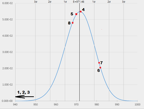
The solid vertical line shows the expected value; the thin vertical lines indicate one, two and three sigmas distance from it in both directions. Red dots correspond to the values from the table above (some were so far away though that they didn’t fit into the picture).
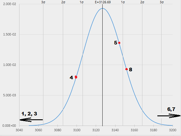
Here are the results for the counts structure (element count 3938, E [Num] = 3126.69, σ [Num] = 20.68), first as a table:
| Label | Hash | Num | Num−E | (Num−E)/σ |
|---|---|---|---|---|
| 1 | Long default | 302 | -2824.69 | -136.52 |
| 2 | Multiply by 3, 5 | 1108 | -2018.69 | -97.57 |
| 3 | Multiply by 11, 17 | 2252 | -901.69 | -43.58 |
| 4 | Multiply by two big primes | 3099 | -27.69 | -1.34 |
| 5 | Multiply by one big prime | 3144 | +17.31 | +0.84 |
| 6 | Modulo big prime | 3236 | +109.31 | +5.29 |
| 7 | CRC32 | 3228 | +101.31 | +4.90 |
| 8 | Random | 3151 | +24.31 | +1.17 |
and as a graph:
In statistics, a three sigma distance from the mean value is usually considered a boundary between likely and unlikely. Normally distributed random variable falls within 3σ from its mean value with probability 99.7%. The probabilities for 1σ and 2σ are 68.2% and 95.4%. Physicists usually require the difference to be 5σ to be really sure that they have discovered something new. That was the achieved confidence in the Higgs boson search.
In our case, we want the opposite – the result to be close to the mean value. The first three hash functions,
as we see, perform very badly, the Long one being the absolute negative champion. No wonder the program ran so slowly.
Our “fast” version, the one multiplying by 3 and 5, however, also turned out to be bad. We’ll need to replace it with
something better. All the other functions seem to behave reasonably well, mostly measuring within 1 – 2σ.
We can see that the random number test gave −0.48σ in one case and 1.17σ in another one, which shows that
such variations are quite achievable by chance.
There are, however, two interesting cases, both for counts, where “modulo big prime” and CRC32 produced exceptionally
good results, both differing from the mean value by over 3σ positively. These points
didn’t even fit into the graph, so far to the right they were positioned. Why this happens and whether it means that
these two hash functions are better then the others for any Life simulation, I don’t know. Perhaps
some mathematically inclined reader can answer this.
These statistics are applicable to Java 7, because the results of hash functions are shuffled the way Java 7 does it. However, the results without shuffling are similar.
Note on the test data
It is important to test the hash functions on realistic input data. For instance, our entire
colony fits into a bounding rectangle sized about 5000×5000, both x and y being below 2500 in absolute value.
It could affect the behaviour of some hash functions (for instance, it is possible that the exceptionally good
results of the division-based function have something to do with it). If we want the hash functions to perform
well on a broader set of inputs than just one test, we must test it on those inputs.
How fast are our hash functions?
Any of the functions from label 4 onwards in the tables above are suitable, with the obvious exception of the random one.
Which one is the best, depends on their own speed – a well-hashing, but slow function is a bad choice.
Let’s measure. We’ll create several versions of the LongPoint class, their names ending with labels from the table above.
We’ll also make special versions of Hash_LongPoint, using those LongPoints. We’ll run the tests on both Java 7 and Java 8.
Various versions of LongPoint only differ in hash function, and could be implemented as classes derived
from LongPoint. However, the amount of re-used code will be very small, hardly worth the effort.
Various versions of Hash_LongPoint only differ in the versions of LongPoint they use. They could
have been implemented as one generic class if they didn’t need to instantiate LongPoint objects. We could work that around
by introducing factory classes, but this would complicate our code and hardly improve performance. This is where C++
templates once again would have worked better than Java generics (I haven’t yet found examples of the opposite).
Here are the results as a table (again, each test was executed on its own):
| Label | Hash | Time, Java 7 | Time, Java 8 |
|---|---|---|---|
| Ref | Multiply by 3, 5 | 2763 | 4961 |
| 1 | Long default | 4273 | 6755 |
| 2 | Multiply by 3, 5 | 2602 | 4836 |
| 3 | Multiply by 11, 17 | 2074 | 2028 |
| 4 | Multiply by two big primes | 2000 | 1585 |
| 5 | Multiply by one big prime | 1979 | 1553 |
| 6 | Modulo big prime | 1890 | 1550 |
| 7 | CRC32 | 10115 | 3206 |
And as a graph:
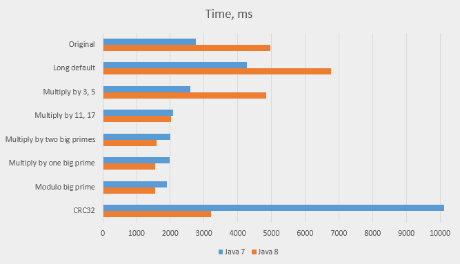
Immediate observations:
-
When hash functions are bad, Java 8 performs worse than Java 7. I can only attribute it to abandoning the bit shuffling in favour of optimising the chains (binary trees instead of lists). The binary tree implementation may become especially slow if chains grow and shrink often – they are then converted from lists to trees and back. This is likely to happen a lot in Life, although I didn’t measure it. In general, I’m not convinced that binary trees were a good idea to begin with. Properly sized arrays and good hash functions should make binary trees unnecessary.
-
The original hash function (multiplying by 3 and 5) is indeed not very good; multiplying by 11 and 17 is better, especially in Java 8; multiplying by two big numbers is even better on both versions.
-
Multiplying by one big prime is so close to multiplying by two big primes that neither has definite advantage.
-
This is the biggest surprise: modulo big prime performs best in both versions of Java. It was above average on the distribution curve (point
6on the graphs), but I didn’t expect good overall results due to the cost of division operation. -
CRC32is slow on Java 8 and very slow on Java 7. The cost of calculating this function seem to defeat all its benefits regarding the quality of hashing, However, there are ways to optimise this function; we’ll look at them in the next article.
Some more statistics
Just out of curiosity I’ve added some counters to our program and got statistics for hash table use:
| Operation | field | counts |
|---|---|---|
put(), new | 1,292,359 | 2,481,224 |
put(), update | 0 | 15,713,009 |
get(), success | 1,708,139 | 48,514,853 |
get(), fail | 1,292,359 | 2,497,339 |
remove() | 1,291,733 | 2,478,503 |
| All operations | 5,584,590 | 71,684,928 |
hashCode() | 77,269,518 | |
The data is collected on a single test run, 10,000 iterations, beginning with ACORN.
The number of hash codes calculated equals the total number of hash map operations, which is expected. In total, the hash was calculated 77 million times, which confirms that hash table operations are indeed the main bottleneck of the program.
In addition, the number of equals() calls on Point object is 160,526,879, or roughly two per hashCode() call,
for the reference implementation, and 36,383,032 (0.47 per hashCode()) for “Modulo big prime”. This is a direct
consequence of the latter version using much better hash function. The reason the number of equals() invocations
per hashCode() is less than one is in unsuccessful get() calls, which are very frequent in Life.
We can also see that much more operations are performed on counts than on field, which is to be expected (eight
lookups and updates are performed for each modification of fields). Any improvement there
will improve the overall speed; the first idea that comes to mind is replacing the immutable Integer values
with mutable ones – this may reduce the number of updating put() calls.
Another idea is more technical. In the following code
for (Point w : counts.keySet ()) {
    if (counts.get (w) == 3 && ! field.contains (w)) toSet.add (w);
}
we call counts.get() on a value that has just been extracted from counts.keySet(). Using the entrySet()
will eliminate the need for get(), reducing the number of operations a bit. We’ll try these (and others) optimisations
later.
Conclusions
-
The quality of hash functions is important. For applications with heavy usage of hash tables, the choice of hash functions can be the single most significant factor determining the performance.
-
The default hash function of
Longisn’t friendly towards packed values. If several values are kept in onelong, and thislongis often used as a hash key, hand-written special classes with well-chosen custom hash functions may work better. The same probably applies toInteger. -
It makes sense to check, and possibly fine-tune, the hash function for the specific case. It mustn’t produce results much worse than the expected value of the Numk random variable. The above formulas can be used to find both the expected value and the variance.
-
There is always a trade-off between quality and speed of hash functions. Sometimes a very good hash function may turn out to be too slow.
-
Time to run the test went down by 32% for Java 7 and 69% for Java 8, compared with the original version (much more if compared with the first
long-based version). Not bad, considering that we didn’t change the algorithm or the data structure – only the hash function. -
The achieved number of iterations per second was 6,451 (it was 3,619 when we started). Let’s set a goal of 10,000 and see if this is achievable on the same computer.
Coming soon
In the next article I’ll try to optimise CRC32 and see if it can be made practically usable. I also want to test the influence
of the hash table size, replace basic types with some mutable classes and check what else can be done to speed up
calculations. Finally, I want to replace Java standard hash tables with custom-made ones and see if that helps.
And I still want to try the glider gun.