In “Game of Life, hash tables and hash codes” we implemented Conway’s game of Life using Java’s HashMap.
We found that performance depends on the choice of a hash function and studied how to measure their quality and speed. We found one hash function that is suitable.
In “Optimising the hash-based Life” we improved the original implementation. It now runs twice as fast as when we started.
The code can be seen in the repository.
Now I’m going to study the effect of the hash map’s capacity.
The naming convention
The HashMap class is backed by an array that contains the roots of the lists of hash map entries (which we’ll call “chains”).
It is tempting to call the size of that array the size of the hash map.
This would, however, be incorrect, since the word size is reserved for the number of elements in the hash map (as returned by the size() method). The correct HashMap
slang for the array size is capacity.
The hash map and its capacity
The underlying array is created and managed by the HashMap class itself, and usually the programmer doesn’t have to bother about this array and its size.
The default constructor of the HashMap sets the capacity to 16; the user may specify another value, which will be
rounded up to the nearest power of two. Another parameter that regulates the capacity is called a loadFactor; it controls how many elements can be inserted into the
table before its array is expanded. The default value is 0.75. When the table size exceeds its capacity multiplied by this factor, the array is doubled in size
and all the elements copied to the new array. The table never shrinks. After some time the capacity stabilises at some reasonable value, which is bigger than the
table size, but not too much bigger.
In our implementations we preferred to avoid array resizing and allocated the tables with the initial capacity of 8192. The initial implementation used two hash maps.
One, called field (actually a HashSet, which is backed by a HashMap), contained the live cells. It reached the maximal size of 1034.
Another one, called counts, contained the numbers of the live neighbours for the cells. This one reached the size of 3938, so the HashMap with the default
capacity would have stabilised at the capacity of 8192 anyway. The field could use smaller table (2048).
The optimised implementation uses just one hash table, called field, which stores objects that contain both cell status (live or not) and their neighbour number.
This table reached the size of 4041. This size is bigger than the highest neighbour count (3938), because the new table contains live cells with neighbour count of zero.
Anyway, this table would also settle at the capacity of 8192.
The default load factor of 0.75 makes sure that the capacity is never too big. The biggest it gets is 8/3 of the table size right after the resize. This approach seems too conservative. Why not use bigger capacity? This is what we’ll study today.
Intuitively it seems that the bigger the capacity, the more efficient is the hash table. The number of comparisons performed for every operation is determined by the chain length (the number of entries sharing the same array slot). If the hash function is not too bad, this chain length must decrease with grows of the capacity. We saw in “Game of Life, hash tables and hash codes” that the random hash function caused the average number of slots used after insertion of 3938 elements to be 3126, which corresponds to the average chain length of 1.259. If we manage to bring this value down close to 1, we can eliminate 20% of all comparisons. It seems obvious that the chain length will approach 1 as we increase the capacity, but it can also be proven formally.
In the same article we’ve produced the formula for the expected value of Numk (the number of used array elements after k insertions):
| E[Numk] = M (1 − (1 − | 1 | ) | k | ) |
| M |
where M is the capacity.
When M grows infinitely, we can approximate the innermost expression with two terms of its binomial expansion:
| (1 − | 1 | ) | k | = 1 − | k | + O ( | 1 | ) |
| M | M | M2 |
After substitution and reduction, we get the following for E[Numk]:
| E[Numk] = k + O ( | 1 | ) |
| M |
The average chain length Lenk is inversely proportional to the number of used slots:
| Lenk = | k |
| Numk |
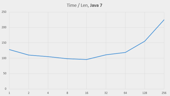
This value approaches 1 as M grows. This is what the behaviour of Lenk looks like for k = 4000:
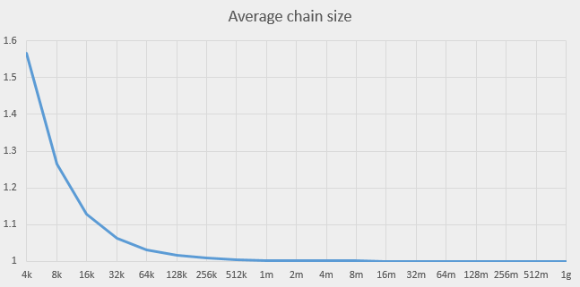
This graph shows that we should be able to do better than with current value 8K. It seems to make sense to increase the capacity to at least 256K, which would make the chain length very close to 1. Further increase of capacity doesn’t promise any improvements.
Of course, other factors such as RAM cache may affect the results. We can’t claim anything about the real impact of the capacity until we measure it. Let’s do it.
Measuring the capacity impact
The HashMap has a constructor that takes both the initial capacity and the load factor. We can give it some ridiculously big load factor (say, ten million), which will
effectively prohibit resizing. The capacity will stay as initialised. All we need is to modify the HashMap allocation:
public static final int HASH_SIZE = 8192;

private HashMap<LongPoint, Value> field =
    new HashMap<LongPoint, Value> (HASH_SIZE);
becomes something like this:
public static final int HASH_SIZE = 4096;

private HashMap<LongPoint, Value> field =
    new HashMap<LongPoint, Value> (HASH_SIZE, 10000000.0f));
Here are the results we get for a range of the capacities (these are the times for 10,000 steps of Life simulation, in milliseconds):
| Capacity | Java 7 | Java 8 |
|---|---|---|
| 1 | 256372 | 1947 |
| 2 | 110658 | 1917 |
| 4 | 52715 | 1915 |
| 8 | 24597 | 1904 |
| 16 | 12032 | 1898 |
| 32 | 6941 | 1838 |
| 64 | 3721 | 1835 |
| 128 | 2432 | 1770 |
| 256 | 1763 | 1490 |
| 512 | 1425 | 1395 |
| 1024 | 1218 | 1161 |
| 2048 | 1104 | 1036 |
| 4096 | 1040 | 923 |
| 8192 | 1020 | 904 |
| 16K | 1089 | 806 |
| 32K | 1268 | 852 |
| 64K | 1640 | 935 |
| 128K | 2476 | 1186 |
| 256K | 3721 | 1602 |
| 512K | 6523 | 2516 |
| 1M | 13795 | 4313 |
| 2M | 26650 | 7916 |
| 4M | 52221 | 15160 |
| 8M | 110515 | 39127 |
| 16M | 228141 | 76980 |
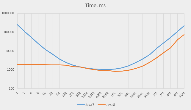
The numbers grow so high that the only way to show both Java 7 and Java 8 results on the same graph is by using the logarithmic scale:
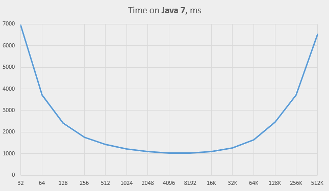
This is the central part of the Java 7 graph (in traditional scale):
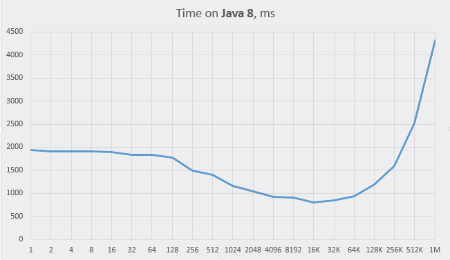
And this is the graph for Java 8:
Here are the three major observations from these graphs:
-
Times on Java 8 are always better than on Java 7 (two to three times in the right side of the graph; much more on the left)
-
Times on Java 7 grow almost to infinity as the capacity decreases, while times on Java 8 do not; the time stabilises at about 128 and stays roughly the same all the way down. The time stays reasonable even when the capacity is set to 1.
-
Times on both versions grow almost linearly on big capacities (above 64K) – contrary to our expectations.
Let’s look at these observations.
The difference in performance at small capacity values
We expect the speed to drop as the capacity decreases, so the behaviour on Java 7 isn’t a surprise. Moreover, the observed times are roughly in accordance with our formula for Lenk (see above). Let’s assume k = 2000 as a representative table size, and plot the value time / Lenk for small values of M for Java 7:
The graph looks almost horizontal up to the capacity of 64, which means that the Java 7 implementation behaves in the expected way.
The Java 8 behaviour is different. It keeps running reasonably fast even when chains become very long. This can only be due to the innovation that has been
introduced in Java 8’s implementation of the HashMap: the binary trees of the entries. When entry lists exceed the length of 8, they are converted to binary trees
with full hash codes as search keys. This conversion takes time, but it improves the speed of the searches. As we see, the speed stays good even at the array size of 1, when
the entire table is stored in just one entry. Effectively, the entire hash map becomes a tree map in this case, which suggests that perhaps we must try this solution as well.
The average chain length (assuming k=2000) is 7.8 at the capacity of 256 and 15.6 at 128, which means that the capacity of 128 is roughly the point where the binary trees start to kick in massively. This is also the point (see the “Time on Java 8” graph above) where the time graph behaviour changes; it becomes roughly horizontal to the left of this point.
The performance at high capacity values
The times grow steadily as the capacity grows above 64K. Two lines on the logarithmic graphs are almost parallel to each other and almost straight, which means that the time is roughly proportional to the capacity. Let’s divide the time by the capacity and plot this value for both Java 7 and Java 8:
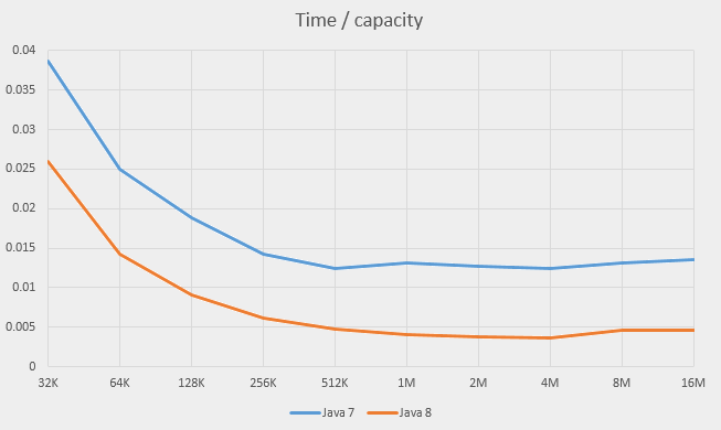
The graph shows that the time is indeed proportional to the capacity, very accurately so starting at approximately 1M elements and less accurately from 256K. The graphs also show slight relative slowdown at 8M - probably, this is the effect of RAM caching.
There is nothing in the basic HashMap operations (get, put or remove) that depends linearly on the capacity (it is the entire purpose of a hash table to avoid
such dependency). However, there is such dependency in iterating the HashMap, and this is something we do in step(). The only way to iterate a hash map is to iterate its
underlying array and for the non-empty elements iterate corresponding chains (linked lists). Starting at some point, iterating over the empty array elements will dominate
everything else. It seems reasonable to collect the HashMap values into some other collection that allows easy insertion and deletion as well as quick iteration.
The linked list is the ideal option.
We don’t need to do it by hand: Java has a standard class with this functionality: LinkedHashMap. The elements of this hash map are linked together in a doubly-linked
list. The main purpose of this class is different, though: it is to iterate the elements of the map in the order they were inserted, which the classic HashMap does not provide.
Still, we can try using this class and check if it helps.
This time we could run tests at bigger capacities – up to 1G:
| Capacity | Old time | New time | ||
|---|---|---|---|---|
| Java 7 | Java 8 | Java 7 | Java 8 | |
| 1 | 256372 | 1947 | 261389 | 2083 |
| 2 | 110658 | 1917 | 108080 | 1855 |
| 4 | 52715 | 1915 | 55500 | 1970 |
| 8 | 24597 | 1904 | 26517 | 1951 |
| 16 | 12032 | 1898 | 12690 | 1969 |
| 32 | 6941 | 1838 | 6643 | 1970 |
| 64 | 3721 | 1835 | 3795 | 1992 |
| 128 | 2432 | 1770 | 2447 | 1710 |
| 256 | 1763 | 1490 | 1728 | 1533 |
| 512 | 1425 | 1395 | 1361 | 1553 |
| 1024 | 1218 | 1161 | 1135 | 1174 |
| 2048 | 1104 | 1036 | 985 | 912 |
| 4096 | 1040 | 923 | 939 | 834 |
| 8192 | 1020 | 904 | 902 | 742 |
| 16K | 1089 | 806 | 878 | 640 |
| 32K | 1268 | 852 | 870 | 651 |
| 64K | 1640 | 935 | 820 | 601 |
| 128K | 2476 | 1186 | 844 | 593 |
| 256K | 3721 | 1602 | 873 | 572 |
| 512K | 6523 | 2516 | 843 | 581 |
| 1M | 13795 | 4313 | 836 | 611 |
| 2M | 26650 | 7916 | 852 | 629 |
| 4M | 52221 | 15160 | 959 | 695 |
| 8M | 110515 | 39127 | 973 | 697 |
| 16M | 228141 | 76980 | 952 | 668 |
| 32M | 892 | 685 | ||
| 64M | 887 | 673 | ||
| 128M | 962 | 748 | ||
| 256M | 1032 | 876 | ||
| 512M | 1336 | 1270 | ||
| 1G | 2146 | 1935 | ||
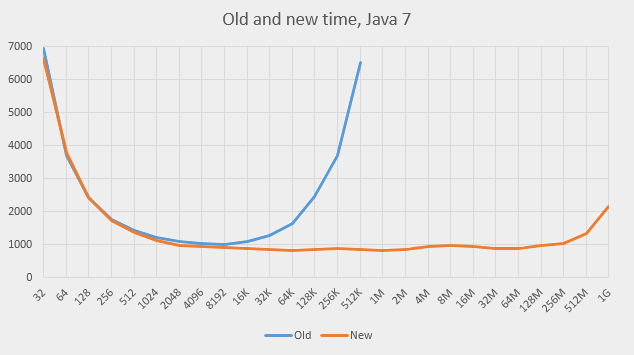
Here are the graphs. This is for Java 7:
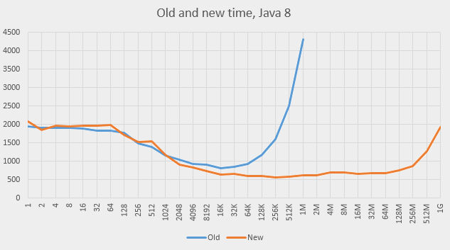
And this is for Java 8:
Some observations:
-
The behaviour at big capacities became much better on both versions of Java. The graphs are nearly flat for a wide range of capacities (512 to 512M). The slowdown was indeed caused by the
HashMapiteration, and introducing the linked list resolved the problem. -
The Java 8 graph is not completely flat at the ends but never goes too high, either. All the capacities are quite usable in Java 8.
-
The behaviour at small capacities is roughly the same as before, mostly a bit slower, which is understandable: the lists do not add any benefit but require time for their maintenance.
-
The program previously ran at the capacity of 8192, which is the value the
HashMapwould have settled upon naturally (the element count is about 4000 and the load factor if 0.75). The added linked lists help there already. In fact, the positive effect of the lists start at capacity 512 on Java 7 and on capacity 2048 on Java 8. -
This means that
LinkedHashMapis always better than ordinaryHashMapwhen the map if often iterated. -
This also explains why the load factor was chosen 0.75 for the standard
HashMap: the designers of that class didn’t know if the map would be iterated, and insured themselves against very slow execution in the case it would. Since theLinkedHashMapis supposed to be iterated (this is its primary purpose), it could use different default load factor. It is strange it doesn’t. -
The best performance is achieved on capacities between 64K and 2M on both systems. The absolute times (roughly 820 and 580 ms) are 20% and 36% better than the best times achieved so far using standard capacity.
-
Both graphs show one step up at about 4M and one incline at 256M. The first one can be explained by the effects of RAM caching (the processor has 20Mb of L3 cache). The second is probably due to the garbage collector costs (the garbage collector scans the entire array to mark used blocks; scanning the empty slots also takes time).
The effect of the garbage collector
The garbage collector theory is easy to verify – we can use the Java command-line option -Xloggc:file to print the garbage collector invocations.
This is what is printed when running on Java 8 with the capacity of 8192 (our test program runs the simulation three times):
0.713: [GC (Allocation Failure)  258048K->984K(989184K), 0.0020325 secs]
1.069: [GC (Allocation Failure)  259032K->1312K(989184K), 0.0038226 secs]
1.338: [GC (Allocation Failure)  259360K->1152K(989184K), 0.0046389 secs]
1.665: [GC (Allocation Failure)  259200K->1010K(989184K), 0.0028201 secs]
1.919: [GC (Allocation Failure)  259058K->1394K(989184K), 0.0069037 secs]
2.229: [GC (Allocation Failure)  259442K->916K(1205760K), 0.0033108 secs]
Six GC invocation take 23ms in total, or 7ms per simulation, or roughly 1% of total execution time, which is reasonable.
Now let’s look at the execution with the capacity 1G:
1.761: [GC (Allocation Failure)  4452352K->4195032K(5184000K), 0.7945753 secs]
3.367: [GC (Allocation Failure)  4453080K->4195216K(5442048K), 0.7838357 secs]
5.528: [GC (Allocation Failure)  4711312K->4195120K(5442048K), 0.7899669 secs]
-
[A side note: I still can't get used to the heap size of 4Gb; I know these days it isn't even considered big, but I still remember the system in development of which I
once took part: its heap was 8K bytes long, or half a million times smaller than now. And this was as recently as 1982! End of the side note]
Here we have three invocations, averaging to 790 ms, which is 41% of total execution time (1935 ms). This means that GC does indeed play a role in the slowdown at super-big capacities.
Here is the graph (in a logarithmic scale) of the total time taken by the GC.
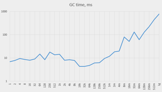
When the capacity is small, the time varies, while staying relatively small compared to the total execution time. Starting at about 1M elements the GC time grows steadily.
This graph shows the absolute values of the total time, the GC time and the pure time (the former minus the latter):
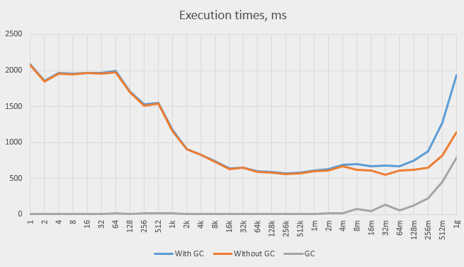
Growth in GC time can’t explain the entire observed increase in total time, but it is responsible for a significant portion of it.
The tree map
We mentioned earlier that Java 8 uses binary trees to represent the chains of HashMap entries that occupy the same slot in the array. What if we replace the HashMap
with a TreeMap? Let’s try it (see TreeLife.java).
Here are the results:
- on Java 7: 2499 ms
- on Java 8: 2841 ms.
Strangely, the result on Java 8 is worse than on Java 7 and worse than when using HashMap of capacity 1.
In any case, the results are bad enough to dismiss the idea.
The best results achieved so far were:
- On Java 7: 820 ms (achieved on the capacity of 64K)
- On Java 8: 572 ms (achieved on the capacity of 256K).
In general, all capacity values between 64K and 1M give good results.
Conclusions
-
The standard capacity of the
HashMapwas chosen with the general use case in mind, which involves occasional iteration. -
Still, if the hash map is iterated often, it is a good idea to rather use the
LinkedHashMap. -
If the hash map is not iterated, or if the
LinkedHashMapis used, it helps to increase the hash map capacity above the standard one; just don’t overdo it. -
We’ve improved the speed by another 20% on Java 7 and 36% on Java 8.
-
The values we started at in the very beginning were 2763 ms for Java 7 and 4961 for Java 8. The overall improvement is 70% for Java 7 and 88% (yes, the 8.5 times speedup) for Java 8.
-
The number of iterations per second reached 12K on Java 7 and 17K on Java 8.
Coming soon
In the next article we’ll check if we can improve speed even more.