I was looking for a simple example problem to demonstrate program optimisation, when I saw a colleague of mine busy with exactly that. He had written a routine for de-multiplexing one complex network protocol on high speed data links and found the performance insufficient – so he was optimising it. By the time I joined the process he had already improved the speed to be sufficient; I managed to make it a bit faster, too. I couldn’t use his problem directly as an example, because it was too complex for that, but it reminded me of a much simpler problem that could demonstrate the same optimisation techniques: the de-multiplexing of E1 streams.
It is a very simple problem indeed. It is very hard to produce a solution longer than twenty lines (I’ll try, however). Yet it is a real-world problem rather than an academic exercise. And, although one may wonder if there is any space for optimisation at all, I’ll show that there is. In short, the problem seems ideal for a starting point of out optimisation journey. Besides, I’m curious: What is the de-multiplexing speed, in megabytes per second, that can be achieved on modern machines using typical programming tools?
In this article I’ll implement and optimise the E1 de-multiplexing in Java. Later I’ll try C/C++ as well.
The entire project is available on Github in a repository: https://github.com/pzemtsov/article-E1-demux-Java
Problem definition
An E1 stream is a network line, most commonly used in digital telephony, capable of carrying 2,048,000 bits per second. This capacity is used to carry 32 streams of 64,000 bits/sec, each of which is sufficient for one side of a telephonic conversation. These individual streams are combined together using a technique called Time Division Multiplexing. This simply means that time is divided into equal portions and these portions are allocated to the streams in round-robin fashion. That’s why component streams of the E1 are called timeslots. Fortunately for us, the unit of transmission was chosen as a very convenient 8 bits, which allows us to view an E1 stream as well as its timeslots as byte streams. The source stream (256,000 bytes/sec) can be considered a sequence of 32-byte frames, where the nth byte of each frame belongs to the nth timeslot. This way each timeslot receives 8,000 bytes per second. These bytes per seconds are not important for the de-multiplexing process itself; I only mention them because I want to compare the speed of our de-multiplexer with the actual speed of the stream.
Let’s assume that our machine is equipped with an E1 card, which sends the source byte stream to our program, one buffer at a time. The card
takes care of frame synchronisation, so we know that the data we receive starts and ends at valid frame boundaries, which makes the data size
a multiple of 32. The input buffer will be modelled as a Java byte array. We need to decompose the input stream into 32 output buffers, which
will also be represented as byte arrays of appropriate size. We’ll ignore the buffer and pointer management, assuming that the output buffers
will be processed immediately after de-multiplexing, and can be re-used straight away.
I’ll also assume that both input and output data are in the processor cache. This is a simplification, but it is appropriate for our little example. To achieve this, I’ll use an input buffer small enough to fit into the cache completely. I’ve chosen a buffer size of 2048 bytes, or 64 bytes per timeslot.
It seems pretty obvious that we should be able to de-multiplex an E1 even in BASIC: as said earlier, the byte rate of an E1 stream is 256,000 bytes/sec, or roughly 4 microseconds a byte. Assuming a typical clock speed of a modern processor to be 2.5GHz, this means that we have 10,000 CPU cycles available to process each incoming byte. We expect much less cycles to be needed for that, so a program in Java must work faster than real time. This doesn’t mean that optimisation is useless: we can de-multiplex more than one E1 stream on one processor core. Let’s see how many we can do.
The reference implementation
We are ready to start coding. We’ll start with the most naïve and straightforward version possible, which we’ll call the reference implementation. The name indicates that both correctness and performance of other implementations will be tested against this one.
To simplify the test framework, all the implementations will be designed as classes implementing the common interface
Demux.
The code is very simple; it iterates over the entire input array and writes bytes, one at a time, to the destination arrays in round-robin fashion, closely
following the logic of a hardware E1 decoder. Here is the code
(see class E1.Reference):
public final class E1
{
    public static final int NUM_TIMESLOTS = 32;
    public static final int DST_SIZE = 64;
    public static final int SRC_SIZE = NUM_TIMESLOTS * DST_SIZE;

    interface Demux
    {
        public void demux (byte[] src, byte[][] dst);
    }

    static final class Reference implements Demux
    {
        public void demux (byte[] src, byte[][] dst)
        {
            assert src.length % NUM_TIMESLOTS == 0;

            int dst_pos = 0;
            int dst_num = 0;
            for (byte b : src) {
                dst [dst_num][dst_pos] = b;
                if (++ dst_num == NUM_TIMESLOTS) {
                    dst_num = 0;
                    ++ dst_pos;
                }
            }
        }
    }
}
The method checks that the input is a multiple of NUM_TIMESLOTS, because it doesn’t work otherwise. First of all, the interface itself relies on the fact
that all the outputs receive the same number of bytes, and that isn’t true for arbitrary input sizes. And secondly, the implementation assumes that the
first byte in each input buffer belongs to output zero (it sets dst_num to 0). Both of these assumptions can be removed by appropriate modifications of
the interface and implementation (I’ll skip the demonstration). This is typical for reference implementations: they are usually more flexible than the
highly optimised ones. You will see that other implementations can’t be modified so easily.
The method does not check sizes of destination arrays but rather relies on a run-time exception being thrown if the arrays are too small.
I especially like the line for (byte b : src) in this code. It uses the iterator syntax, which was added to Java relatively late (in version 1.5),
and which has great value in making programs look nicer. Here the loop written using such syntax immediately makes it clearly visible that the entire
src array is iterated in the natural order of elements, and that its elements are only read and not written. It is very appropriate for a reference
implementation.
This method is 13 lines long, well within the 20 line budget that I mentioned earlier.
Test framework
We are still not ready to run the test implementation. We need to create a test framework first.
We need methods to create the test input data and to allocate the test outputs:
static byte[] generate ()
{
    byte [] buf = new byte [SRC_SIZE];
    Random r = new Random (0);
    r.nextBytes (buf);
    return buf;
}

static byte[][] allocate_dst ()
{
    return new byte [NUM_TIMESLOTS][DST_SIZE];
}
The generate () method fills the allocated array with pseudo-random numbers. Note that Random object is initialised with the seed value of 0. As a result,
we get the same sequence of “random” numbers each time we run this method. It won’t make any difference for E1 decoding, but it is a good practice to use
in other cases, where the speed may depend on the input data (a classic example is the array sorting problem).
Next, we need a performance measuring code:
public static final int ITERATIONS = 1000000;
public static final int REPETITIONS = 5;

static void measure (Demux demux)
{
    byte[] src = generate ();
    byte[][] dst = allocate_dst ();

    System.out.print (demux.getClass ().getCanonicalName () + ":");

    for (int loop = 0; loop < REPETITIONS; loop ++) {
        long t0 = System.currentTimeMillis ();
        for (int i = 0; i < ITERATIONS; i++) {
            demux.demux (src, dst);
        }
        long t = System.currentTimeMillis () - t0;
        System.out.print (" " + t);
    }
    System.out.println ();
}
And the main method:
public static void main (String [] args)
{
    measure (new Reference ());
}
(the entire test and measurement code can be seen here).
The execution time is printed in milliseconds, because such is the resolution of the standard Java timer.
I like it when execution time is between 500 ms and 10,000 ms. It is long enough to allow sufficient measurement accuracy
but short enough not to get bored. In our case this can be achieved by setting the ITERATIONS parameter to one
million.
As is visible from the code, we don’t just repeat the method execution one million times but also repeat the entire
measurement five times (the value of REPETITIONS). This is done to handle the effect known as
HotSpot warm-up. When the Java VM starts executing a program, the byte code
is interpreted directly. This is very, very slow. While this happens, the VM collects execution statistics and detects
code sections where most processor time is spent (hot spots, which gave name to Java’s JIT compiler).
These sections are then compiled into native code and optimised. The process of compiling also uses CPU time, so usually
the performance of Java programs isn’t great at start-up but improves later. We are interested in stable results on
well warmed-up HotSpot, that’s why we run several iterations.
First results
After all the preparations, we are finally ready to run the program. I’m going to use the server VM of Java version 1.7_40 on Linux, running on a Dell blade with Intel® Xeon® CPU E5-2670 @ 2.60GHz.
# Java -server E1
E1.Reference: 2897 2860 2860 2860 2860
The effect of HotSpot warm-up is visible, but it is quite small. The execution times starting from the second iteration are remarkably stable. Are they also stable between runs? Let’s run it again
# Java -server E1
E1.Reference: 2909 2860 2859 2860 2860
The results, as measured after the warm-up, are still stable. We needn’t bother with running the program multiple times, provided that the computer conditions are consistent between running different tests (clock frequency and memory configuration are the same, the same version of OS is running and no one else is running other tests at the same time).
Just out of curiosity: how much does the HotSpot increase the speed of execution compared to interpreting of the byte code? Java has a special switch to turn HotSpot off:
# java -Xint -server E1
E1.Reference: 44623 44581 44583 44584 44583
The HotSpot does a really good job!
Let’s return to our result obtained with HotSpot on: 2,860 ms. How good is this result? Is the speed sufficient for practical needs? To answer this, we must recall that we measure time for 1,000,000 iterations, each time decoding a buffer of 2048 bytes, which results with the volume processed each second to be 1000000 * 2048 * 1000 / 2860 = 716M bytes (I’m using the metric megabyte, which is exactly 1,000,000 bytes). Recalling also that the speed of E1 stream it 256,000 bytes/sec, we can calculate that our de-multiplexing speed is roughly 2,800 times faster than the transmission speed. In ideal world this would have meant that we could process 2800 streams in real time on one processor core, but the reality, as usual, is far from ideal, and the number will be somewhat less. One reason is that 2800 source buffers won’t fit into the processor cache, so our caching pre-condition won’t be met. Let’s leave exact measurements of this effect for later articles.
The speed we achieved is very impressive, probably sufficient for any practical application. This means that we can stop the optimisation exercise right here. But I’d like to carry on, for three reasons. Firstly, any tricks we discover may be helpful for other de-multiplexing problems, and some of them are much more performance-demanding. Secondly, we can learn something of general value, not limited to de-multiplexing. And thirdly, I am still curious: Can it be made faster?
Correctness check
Before writing other implementations, we must add something to our test framework: the basic correctness test. There
is no use comparing performance of two methods if we are not sure they are doing the same thing (I admit that for our super-simple
problem it sounds a bit paranoid, but who knows?). We’ll compare results of all our new methods with the results of the Reference:
static void check (Demux demux)
{
    byte[] src = generate ();
    byte[][] dst0 = allocate_dst ();
    byte[][] dst = allocate_dst ();
    new Reference ().demux (src, dst0);
    demux.demux (src, dst);
    for (int i = 0; i < NUM_TIMESLOTS; i++) {
        if (! Arrays.equals (dst0[i], dst[i])) {
            throw new java.lang.RuntimeException ("Results not equal");
        }
    }
}
We must still not forget to call this method from measure ().
Source-first solutions
The reference implementation represents a source-first approach, where the iteration runs along the source array rather than along the destination. The input data is read sequentially, but the output is written in a scattered way, one byte at a time. Before trying other approaches, I’d like to see what we can achieve without changing the order of memory access. For this I’ll create a source-first family of solutions.
Let’s recall the main loop of the Reference implementation:
for (byte b : src) {
    dst [dst_num][dst_pos] = b;
    if (++ dst_num == NUM_TIMESLOTS) {
        dst_num = 0;
        ++ dst_pos;
    }
}
We can see that dst_num is initially set to 0 and is incremented in the loop until it reaches NUM_TIMESLOTS-1. Then it is set to zero and incremented
again – just as if we were running an inner loop inside the main loop. Effectively, this is what we are doing, only the inner loop is written in an
obscure way rather than directly using the loop statement.
Let’s try writing it directly (here is the code):
static final class Src_First_1 implements Demux
{
    public void demux (byte[] src, byte[][] dst)
    {
        assert src.length % NUM_TIMESLOTS == 0;

        int src_pos = 0;
        int dst_pos = 0;
        while (src_pos < src.length) {
            for (int dst_num = 0; dst_num < NUM_TIMESLOTS; ++ dst_num) {
                dst [dst_num][dst_pos] = src [src_pos ++];
            }
            ++ dst_pos;
        }
    }
}
Running it, we get the following:
# Java -server E1
E1.Src_First_1: 2533 2482 2482 2482 2481
And our results for Reference were:
E1.Reference: 2897 2860 2860 2860 2860
We can see the improvement of 380 ms (13%).
Looking closely at the code of Src_first_1, we see that we increment src_pos in each iteration of the inner loop,
together with dst_num, and we also increment dst_pos in the outer loop. This is excessive, for we maintain three
variables, which are not independent. It is easy to see that these variables maintain the invariant relationship:
src_pos = dst_pos * NUM_TIMESLOTS + dst_num
Why not try replacing src_pos with the expression on the right hand side? The outer loop then runs on dst_pos,
and we mustn’t forget to use the correct loop limit. Since the loop variable isn’t modified inside the loop anymore,
we can replace the while loop with a for loop, which is my personal aesthetic preference. Strictly speaking,
Java does not have a true for loop in the same sense as Pascal has – its for is just another syntax for while.
However, I prefer to follow a convention that for loop contains a dedicated loop variable (or variables) with
explicit initialisation step, increment step, and loop condition, all specified in the loop header. The variable
mustn’t be modified anywhere else. This convention doesn’t forbid emergency loop termination using break, though.
static final class Src_First_2 implements Demux
{
    public void demux (byte[] src, byte[][] dst)
    {
        assert src.length % NUM_TIMESLOTS == 0;

        for (int dst_pos = 0; dst_pos < src.length/NUM_TIMESLOTS; ++ dst_pos) {
            for (int dst_num = 0; dst_num < NUM_TIMESLOTS; ++ dst_num) {
                dst [dst_num][dst_pos] = src [dst_pos*NUM_TIMESLOTS + dst_num];
            }
            ++ dst_pos;
        }
    }
}
Let’s run it:
# java -server E1
Exception in thread "main" java.lang.RuntimeException: Results not equal
Oops! I did something wrong. The modification was not correct, and we can easily see why: I moved the updating of
dst_pos inside the header of the loop but forgot to remove it from the loop body. And the sad part of it is that
I didn’t insert this episode here just to highlight the importance of the correctness testing. This really happened
to me while preparing this article. Fortunately for me, the correctness check was in place (but for a code this simple
the bug should have been detected during code inspection; it could even be done on a formal grounds of violation of the
convention mentioned above).
What would have happened if the check was not there? Let’s comment out the call of check() in measure() and see
what happens:
# java -server E1
E1.Src_First_2: 1205 1168 1167 1168 1166
The code seems twice as efficient as Src_First_1 – but we know now that it only does half the work, since it
increments the loop variable twice in the loop!
Let’s fix the error and run the test again:
static final class Src_First_2 implements Demux
{
    public void demux (byte[] src, byte[][] dst)
    {
        assert src.length % NUM_TIMESLOTS == 0;

        for (int dst_pos = 0; dst_pos < src.length/NUM_TIMESLOTS; ++ dst_pos) {
            for (int dst_num = 0; dst_num < NUM_TIMESLOTS; ++ dst_num) {
                dst [dst_num][dst_pos] = src [dst_pos*NUM_TIMESLOTS + dst_num];
            }
        }
    }
}
And here is the result:
# Java -server E1
E1.Src_First_2: 2324 2285 2287 2284 2284
I remind you that the previous result was:
E1.Src_First_1: 2533 2482 2482 2482 2481
Src_First_2 shows improvement by about 200 ms, or 8.8% over Src_First_1.
What I’ve done in Src_First_2 is the reversal of a well-known program transformation often performed by optimising
compilers, called operation strength reduction.
The compiler detects induction variables (those that are
incremented in a loop by constant values), and if they are multiplied by constant values inside the loop, replaces
the results of such multiplications with another, synthesised induction variables. Here I’ve done exactly the opposite,
and, strangely, it improved the speed. Most likely, the HotSpot compiler performs this transformation, and does it
better than we can do manually.
Now we’ll try a completely different approach in running the loops. For each index in the source array we can calculate where exactly the byte from that index must go. This way we only need one loop. Here is a new version:
static final class Src_First_3 implements Demux
{
    public void demux (byte[] src, byte[][] dst)
    {
        assert src.length % NUM_TIMESLOTS == 0;

        for (int i = 0; i < src.length; i++) {
            dst [i % NUM_TIMESLOTS][i / NUM_TIMESLOTS] = src [i];
        }
    }
}
Here are the results:
# Java -server E1
E1.Src_First_3: 4405 4359 4360 4360 4360
This is impressive – the speed has dropped almost by half from Src_First_2. The explanation of this fact requires
analysis of the machine code generated by HotSpot. Without looking at that code I can only speculate. Variable i
is an induction variable, but i % NUM_TIMESLOTS and i / NUM_TIMESLOTS are not. The compiler can’t easily replace
them with any other easily maintainable variables, so it has to perform both division and modulo operations.
Since NUM_TIMESLOTS equals 32, these operations can be done fast (modulo is done by a single AND instruction
and division is a shift), but even one extra instruction inside a loop can make a difference. Another possible
source of the slowdown is the array index checking. Most compilers optimise index checking for cases where indices
are induction variables. If the first and the last value of such variable are known, a compiler can test only those
values for validity as array indices before entering the loop and avoid checking indices inside the loop. If the
indices aren’t induction variables then the compiler is unable to perform this optimisation.
We’ve looked at four versions of the source-first implementations. We started with the reference implementation,
which was acceptable, improved the speed a bit in Src_First_1 and then in Src_First_2 (in total by about 20%
over Reference), and the final attempt with Src_First_3 failed completely, being much slower than even Reference.
It’s time to finish with the source-first and start looking for other options.
Destination-first solutions
Since our de-multiplexer processes the entire input buffer, it doesn’t have to process bytes in their natural order, which is the order of their arrival on an E1 line. The data can be transferred in any order, and there are 2048! ways to order 2048 elements, which is roughly 1.67*105894. I can think of two reasons why some orders can be better than others. The first reason is that the order of memory reads and writes can affect performance, and the second is that different structure of iterations can cause the compiler to generate better code.
I think the effect of memory access order is unlikely to be big – after all, we deliberately made the input buffer small enough to fit into the cache. The processor has several levels of cache, the fastest of them being also the smallest – level 1 cache. Our processor belongs to the Sandy Bridge family and has the level 1 (L1) data cache of 32 Kbytes. That’s more than enough for the entire input buffer, all output buffers and all the references. However, cache bank conflicts may cause some uncached memory access even when there is cache space available. That’s why some effect of memory access re-ordering is possible, but the difference in code generation has more chances to affect the speed.
Out of the vast number of possible byte ordering, we’ve tried one (iterating along the source array). The most natural other order to try is the destination-first ordering. We’re going to take one output array, fill it up in its natural order, take the next one, etc.
The Src_First_2 class can be easily modified to iterate along destination arrays – all that’s needed is to change
the order of the loops. Here is the code:
static final class Dst_First_1 implements Demux
{
    public void demux (byte[] src, byte[][] dst)
    {
        assert src.length % NUM_TIMESLOTS == 0;

        for (int dst_num = 0; dst_num < NUM_TIMESLOTS; ++ dst_num) {
            for (int dst_pos=0; dst_pos < src.length/NUM_TIMESLOTS; ++dst_pos){
                dst [dst_num][dst_pos] = src [dst_pos*NUM_TIMESLOTS + dst_num];
            }
        }
    }
}
Running it, we get this:
# Java -server E1
E1.Dst_First_1: 1205 1154 1155 1154 1155
The highest speed we achieved before was that of Src_First_2, which took 2284 ms, and the new method runs almost
twice as fast! I think most of the improvement is due to different code generated by the compiler. Specifically,
I think, what made a difference is the fact that dst[dst_num] is now invariant in the inner loop and can be moved
out of it. However, the different order of memory access
may also have played a role, but checking it requires additional experiments. I’ll skip them to keep this article
short but return to this issue in one of the later articles.
The code of Dst_First_1 contains some features that seem inefficient. Apart from the earlier mentioned indexing
of dst [dst_num], the inner loop contains calculation src.length / NUM_TIMESLOTS, which also
does not depend on the loop variable and can be moved out of the loop. In addition, dst_pos is an induction variable,
and its multiplication by NUM_TIMESLOTS can be replaced by addition. A good compiler will do all of that itself.
But is our compiler good?
Let’s test it. Here is the code:
static final class Dst_First_2 implements Demux
{
    public void demux (byte[] src, byte[][] dst)
    {
        assert src.length % NUM_TIMESLOTS == 0;

        int dst_size = src.length / NUM_TIMESLOTS;
        for (int dst_num = 0; dst_num < NUM_TIMESLOTS; ++ dst_num) {
            byte [] d = dst [dst_num];
            int src_pos = dst_num;
            for (int dst_pos = 0; dst_pos < dst_size; ++ dst_pos) {
                d[dst_pos] = src[src_pos];
                src_pos += NUM_TIMESLOTS;
            }
        }
    }
}
Running the method, we get the following:
# Java -server E1
E1.Dst_First_2: 2109 2094 2094 2097 2093
Dst_First_2 is remarkably slower than Dst_First_1. The compiler seems to be sending a clear message:
“Don’t mess with me, I know better”. Still, the difference is surprisingly big. Without looking at the
generated machine code, I can’t make any realistic explanation of such a difference. It is a mystery,
and maybe I’ll return to it later.
Until now all the methods we’ve been testing were generic: they accepted inputs of any size as long as that
size was a multiple of NUM_TIMESLOTS. But in reality we know this number. The input buffer has the size
of 2048 (SRC_SIZE), and each of the output buffers has the size of 64 (DST_SIZE). Can we gain anything by
hard-coding those values in the method? Let’s take Dst_First_1 and replace the loop upper limit with a
constant (we’ll replace the assert statement as well).
Here is the code:
static final class Dst_First_3 implements Demux
{
    public void demux (byte[] src, byte[][] dst)
    {
        assert src.length == NUM_TIMESLOTS * DST_SIZE;

        for (int dst_num = 0; dst_num < NUM_TIMESLOTS; ++ dst_num) {
            for (int dst_pos = 0; dst_pos < DST_SIZE; ++ dst_pos) {
                dst [dst_num][dst_pos] = src [dst_pos*NUM_TIMESLOTS + dst_num];
            }
        }
    }
}
# Java -server E1
E1.Dst_First_3: 1068 1021 1022 1022 1022
The time went down from 1155 to 1022, which is not insignificant: 11.5%. Again, I can only speculate why it became so much faster. At first, it looks surprising that there is any difference at all. The calculation of the upper boundary of the outer loop was, most likely, moved out of the loop. The result must be stored in a variable, which was, most likely, kept in a register. There isn’t a shortage of general-purpose registers: Intel x64 processors have 16 of them, way more than we can possibly need for this method. Operations with registers are as fast as operations with constants – in short, there shouldn’t be any difference. I think, the difference is in the overall loop organisation. A compiler can generate a loop that runs known constant number of times more efficiently than a loop that runs unknown number of times. For instance, the latter must contain code to check if the number of times is zero. If it is known that the loop runs an even number of times, the loop can be unrolled – replaced by a loop that contains the body twice but runs half the number of iterations. This way we save on the number of loop control instructions. It is more difficult to unroll a loop with arbitrary number of iterations because the compiler has to deal with the “leftovers” in the case the number of iterations is odd.
In short, constant sizes of loops help improving performance, but at a cost of limited applicability of a solution. It’s a choice that the programmer must make.
We’ve looked at three versions of the code written in destination-first fashion. The very first implementation already
demonstrated great improvements over the fastest source-first solution: 49.4%. The attempt to help the compiler with petty
optimisations (Dst_First_2) failed, while hard-coding the buffer size gained additional 11.5%.
Going unrolled
In the previous chapter I mentioned an optimisation called loop unrolling. Most compilers can perform some level of unrolling, typically by factor of 2, less often by factor of 4. Small loops may be unrolled fully – replaced by the appropriate number of copies of the loop body. Compilers usually avoid complete unrolling of big loops, because there are valuable resources associated with the code size – namely, L1 code cache and micro-operation cache. Both caches keep executable machine code, the former in its source form (CPU instructions), and the latter as decoded micro-operations. When a tight loop of frequently executed routine doesn’t fit into the cache, its code has to be read from higher-level cache or primary memory, and, possibly, decoded again, which slows down execution. The same will happen if we have two frequently executed routines, each of which is bigger than half the cache size. The compilers do not know the exact pattern of execution, so they try to avoid this risk by using the code cache sparingly and not generate excessively long code. In addition, the code cache size varies. Sandy Bridge has the size of 32 Kbytes, but older processors had smaller caches.
Manual unrolling of loops adds another problem: the code becomes much less readable and difficult to modify. Imagine you’ve made a bug in the loop body and now have to fix it 64 times. Or maybe you have to double the buffer size and, accordingly, double the iteration count. All of that is very painful and expensive. That’s why deep loop unrolling must be used as your last resort, when you really need the ultimate performance, and after you carefully took all the factors into account.
All that said, I want to create a new family of implementations based on Dst_First: the Unrolled. At first,
I’ll unroll the inner loop fully:
static final class Unrolled_1 implements Demux
{
    public void demux (byte[] src, byte[][] dst)
    {
        assert NUM_TIMESLOTS == 32;
        assert DST_SIZE == 64;
        assert src.length == NUM_TIMESLOTS * DST_SIZE;

        for (int j = 0; j < NUM_TIMESLOTS; j++) {
            final byte[] d = dst[j];
            d[ 0] = src[j+32* 0]; d[ 1] = src[j+32* 1];
            d[ 2] = src[j+32* 2]; d[ 3] = src[j+32* 3];
            d[ 4] = src[j+32* 4]; d[ 5] = src[j+32* 5];
            d[ 6] = src[j+32* 6]; d[ 7] = src[j+32* 7];
<skip>
            d[60] = src[j+32*60]; d[61] = src[j+32*61];
            d[62] = src[j+32*62]; d[63] = src[j+32*63];
        }
    }
}
The inner loop here is fully unrolled. I wrote a program to generate the code – I was too lazy to type it manually.
I don’t include the generator program here because it is straightforward. All other unrolled versions are generated
as well. I didn’t include the code here fully: the <skip> mark indicates where there is more code. The file in the
repository contains the full source.
I left the multiplications, because Java performs constant calculations at compile time, and this way the code looks
clearer. I’ve also renamed variable dst_pos as simply j, to make the text use less space on the screen (it doesn’t
affect execution speed or code size). Also please note two additional asserts: the code is generated for specific
values of NUM_TIMESLOTS and DST_SIZE and won’t work if they are changed. Unfortunately, Java doesn’t have any
macro-features. I can, of course, generate a Java class on the fly and load it, but this is too complex for our
purposes. Some compile-time code generation similar to that of a macro assembler would really have helped here.
Now let’s run it:
# Java -server E1
E1.Unrolled_1: 707 659 658 659 659
That was really worth the effort! The code runs 35% faster than before. Loop unrolling is definitely a useful trick.
How about unrolling the outer loop as well? We can’t expect improvement of the same magnitude. Each loop control instruction from the inner loop executes 2048 times; similar instruction from the outer loop executes 32 times. The effect of removing of the outer instructions is 64 times less than the effect from the inner ones. This is a theory. Let’s see if it is correct. Here is a version that unrolls both loops:
static final class Unrolled_2_Full implements Demux
{
    public void demux (byte[] src, byte[][] dst)
    {
        assert NUM_TIMESLOTS == 32;
        assert DST_SIZE == 64;
        assert src.length == NUM_TIMESLOTS * DST_SIZE;

        byte[] d;
        d = dst[0];
        d[ 0] = src[   0]; d[ 1] = src[  32];
        d[ 2] = src[  64]; d[ 3] = src[  96];
        d[ 4] = src[ 128]; d[ 5] = src[ 160];
        d[ 6] = src[ 192]; d[ 7] = src[ 224];
<skip>
        d = dst[31];
<skip>
        d[60] = src[1951]; d[61] = src[1983];
        d[62] = src[2015]; d[63] = src[2047];
    }
}
Again, I don’t show the whole method, as it is 553 lines long – too long for this article (lines are wider in the repository, otherwise it would be even longer). This proves that it is really possible to write a very long program for a simple task if you try hard enough. How fast does this version run?
# Java -server E1
E1.Unrolled_2_Full: 15935 15880 15883 15887 15867
Oops! Something went wrong. I expected that it might get slower because of the shortage of code cache, but not twenty
times slower! The slowdown seems similar to the one we observed when running Reference with HotSpot switched off.
Perhaps HotSpot panicked when it saw a single method of such a great size, and didn’t compile it at all.
To check it, let’s try running Unrolled_2_Full with -Xint:
# java -Xint -server E1
E1.Unrolled_2_Full: 16586 16548 16557 16551 16553
This proves the point that big methods are not compiled by HotSpot. But we can split a big method into many small methods. The HotSpot will inline some of them, so hopefully not all the call instructions will be actually present in the code. The code, however, looks incredibly ugly:
static final class Unrolled_3 implements Demux
{
    public void demux (byte[] src, byte[][] dst)
    {
        assert NUM_TIMESLOTS == 32;
        assert DST_SIZE == 64;
        assert src.length == NUM_TIMESLOTS * DST_SIZE;

        demux_00 (src, dst[ 0]);
        demux_01 (src, dst[ 1]);
<skip>
        demux_30 (src, dst[30]);
        demux_31 (src, dst[31]);
    }

    private static void demux_00 (byte[] src, byte[] d)
    {
        d[ 0] = src[   0]; d[ 1] = src[  32];
        d[ 2] = src[  64]; d[ 3] = src[  96];
<skip>
        d[60] = src[1920]; d[61] = src[1952];
        d[62] = src[1984]; d[63] = src[2016];
    }
<skip>
    private static void demux_31 (byte[] src, byte[] d)
    {
        d[ 0] = src[  31]; d[ 1] = src[  63];
        d[ 2] = src[  95]; d[ 3] = src[ 127];
<skip>
        d[60] = src[1951]; d[61] = src[1983];
        d[62] = src[2015]; d[63] = src[2047];
    }
}
The entire piece of code takes 649 lines. Running it, we get the following:
# Java -server E1
E1.Unrolled_3: 1064 790 791 789 790
This is slower than 659 ms obtained using Unrolled_1. Possibly, we have hit a code cache size limitation.
We can try reducing code size. In Unrolled_3 it is clearly visible that all demux_xx methods are very similar.
They differ from each other only in indexing of the src array. We can make the offset into this array a method
parameter. There will be one extra addition operation when indexing the array but I hope it will be absorbed by
the addressing mode of memory access instruction, or maybe get removed completely by eliminating common sub-expression
&(src[0])+i (I used C notation here, for Java has no pointer arithmetic).
Here is the code:
static final class Unrolled_4 implements Demux
{
    public void demux (byte[] src, byte[][] dst)
    {
        assert NUM_TIMESLOTS == 32;
        assert DST_SIZE == 64;
        assert src.length == NUM_TIMESLOTS * DST_SIZE;

        demux_0 (src, dst[ 0],  0);
        demux_0 (src, dst[ 1],  1);
        demux_0 (src, dst[ 2],  2);
<skip>
        demux_0 (src, dst[31], 31);
    }

    private static void demux_0 (byte[] src, byte[] d, int i)
    {
        d[ 0] = src[   0+i]; d[ 1] = src[  32+i];
        d[ 2] = src[  64+i]; d[ 3] = src[  96+i];
<skip>
        d[60] = src[1920+i]; d[61] = src[1952+i];
        d[62] = src[1984+i]; d[63] = src[2016+i];
    }
}
And the result is:
# Java -server E1
E1.Unrolled_4: 773 710 710 711 711
This is faster than the previous one (790) but still slower than Unrolled_1 (659). This means that we mustn’t fully
discard this approach, and in some cases it may be productive. It may even be faster on some other processors.
However, in our specific case on our processor a simple loop unrolling gave the best results so far.
Another approach to loop unrolling is partial unrolling. The outer loop in Unrolled_1 runs for 32 iterations,
variable j being incremented from 0 to 31. We can run the loop for 16 iterations, incrementing the variable by
two each time. We’ll have to duplicate the loop body, and process outputs j and j+1 in the same iteration.
If this is not enough, we can duplicate the body 4, 8 or 16 times. Duplicating it 32 times is what we’ve already
tried in Unrolled_2_Full. The loop body was too long, and the attempt failed miserably. I’ve made four versions:
Unrolled_1_2, Unrolled_1_4, Unrolled_1_8 and Unrolled_1_16, the last number in a name indicating the
duplication count. I’ll show only Unrolled_1_2 here but
the code for all four is available in the code repository:
static final class Unrolled_1_2 implements Demux
{
    public void demux (byte[] src, byte[][] dst)
    {
        assert NUM_TIMESLOTS == 32;
        assert DST_SIZE == 64;
        assert src.length == NUM_TIMESLOTS * DST_SIZE;

        for (int j = 0; j < NUM_TIMESLOTS; j+=2) {
            byte[] d;
            d = dst[j];
            d[ 0] = src[j+32* 0]; d[ 1] = src[j+32* 1];
            d[ 2] = src[j+32* 2]; d[ 3] = src[j+32* 3];
<skip>
            d[62] = src[j+32*62]; d[63] = src[j+32*63];

            d = dst[j+1];
            d[ 0] = src[j+1+32* 0]; d[ 1] = src[j+1+32* 1];
<skip>
            d[60] = src[j+1+32*60]; d[61] = src[j+1+32*61];
        }
    }
}
Here are the results:
# Java -server E1
E1.Unrolled_1_2: 711 654 654 655 654
E1.Unrolled_1_4: 748 637 636 637 636
E1.Unrolled_1_8: 850 636 636 636 637
E1.Unrolled_1_8: 853 639 640 639 640
E1.Unrolled_1_16: 25942 25919 25905 25877 25904
Clearly, the Unrolled_1_16 is a failure similar to the Unrolled_2_Full. The others demonstrate some (fairly small)
improvement over Unrolled_1, which took 659 ms. The best of them is Unrolled_1_4, which took 636 ms and demonstrated
an improvement by 23 msec, or 3.5%. It is up to the programmer to decide if such an improvement is worth the effort.
It is important to remember that these figures are obtained in purified example and do not guarantee good performance in real life, where the thread does not just execute the optimised routine infinitely, but also does something else in between. Code cache contention can invalidate all the benefits of loop unrolling.
Possible further improvements
In the Dst_First family of solutions we write consecutive bytes using byte-transfer operations. But the processor can
transfer longer pieces of data: words of two bytes, double words of 4 bytes, quad words of 8 bytes. SSE
instructions can also manipulate 16 bytes at a time and
AVX instructions can do 32. We could accumulate the
appropriate number of bytes and then write them all at once. Unfortunately, Java does not allow it, except when
direct byte buffers are used, and use of these buffers requires an interface change and a total rework of all
the existing solutions. We can’t afford it at this stage.
However, this approach is easy to implement in other languages, such as C, and I was going to check the speed in C anyway. Let’s keep this option in mind.
Results
Let’s put all the results into one table. I’ve used the last result of each test. The last column shows execution
times as percentages of the time or the Reference solution.
| Version | Comment | Time | Rel.Ref |
|---|---|---|---|
| Reference | Strictly follows hardware decoder | 2860 | 100.0% |
| Src_First_1 | Refactored the inner loop of Reference | 2481 | 86.7% |
| Src_First_2 | Nested loops with multiplication | 2284 | 79.9% |
| Src_First_3 | Loop along source with division and modulo | 4360 | 152.4% |
| Dst_First_1 | Nested loops with multiplication | 1155 | 40.4% |
| Dst_First_2 | Dst_First_1 optimised manually | 2093 | 73.2% |
| Dst_First_3 | Dst_First_1 with hard coded input size | 1022 | 35.8% |
| Unrolled_1 | Inner loop unrolled fully | 659 | 23.0% |
| Unrolled_1_2 | Outer loop unrolled by 2 | 654 | 22.9% |
| Unrolled_1_4 | Outer loop unrolled by 4 | 636 | 22.2% |
| Unrolled_1_8 | Outer loop unrolled by 8 | 637 | 22.3% |
| Unrolled_1_16 | Outer loop unrolled by 16 | 25904 | 905.7% |
| Unrolled_2_Full | Both loops unrolled in one huge method | 15630 | 546.5% |
| Unrolled_3 | Both loops unrolled; each iteration of an outer loop made into separate method | 790 | 27.6% |
| Unrolled_4 | Both loops unrolled; all methods from
Unrolled_3 merged into one using parameters | 711 | 24.9% |
Here are the same results as a graph (I removed the worst performers to improve the resolution of the rest):
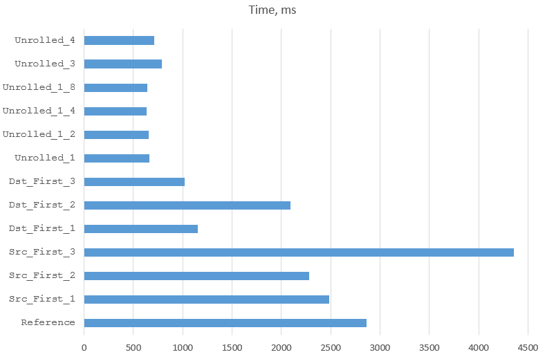
The speeds we have achieved are miles away from those we saw in the beginning. The byte decoding rate is very impressive: 3.2 GBytes/sec, which theoretically allows de-multiplexing of 12,500 E1 streams on one core. The clock speed of our processor is 2.6GHz, which means that the program uses 0.81 CPU cycles to move each byte. Not bad for Java.
What is my personal choice? This depends on the required performance. If the speed of Reference is good enough,
I would use it and not bother with the rest. If we want it faster, I’d use Dst_First_1. Only if the performance
is really critical, my choice would be Unrolled_1. I wouldn’t use any of the highly unrolled solutions,
because I’m not a performance freak.
Conclusions
This is where the Java part of the E1-demultiplexing story ends. Let’s summarise what we learned along the way:
-
There is something to optimise even for such a simple task
-
We managed to speed up the program execution from about 2860 ms to about 640 ms
-
HotSpot does not optimise huge methods, so avoid them
-
The order of iterations is important. In our case iterating the output arrays worked twice as fast as iterating over the source array
-
Reorganising the code while keeping the iteration order also helps, which means that the optimising power of the compiler is limited
-
The compiler is good with simple things like common sub-expression elimination, moving invariant code out of loops, operation strength reduction, etc. Trying to help the compiler to do this kind of work often makes things slower
-
Any performance-orientated changes must be tested; theoretical assumptions about the speeds of different constructs may be wrong
-
Method inlining and loop unrolling help improve speed, but make the code very ugly, especially in Java where there aren’t any meta-programming features. It is often worthwhile looking for some compromise solution, such as partial unrolling. Careful performance testing is needed
-
Whatever you do to improve performance – test the correctness as well!
Notes for myself
These are the items that fell out of the scope of this article but still require some attention. I’ve left them for the future:
-
Why is the speed difference between
Dst_First_1andDst_First_2so big? -
Why destination-first solutions are faster than source-first?
-
What happens if the source buffer does not fit into L1 cache?
-
What happens if we process more than one stream in parallel?
-
Will loop unrolling still be efficient if there is some other code used together with this code?
-
How will the performance be affected if we replace Java arrays with byte buffers?
Coming soon
Will the program run faster if converted to C? Are there better ways to optimise, available in C only? What happens if write the code in C and call in from Java using JNI? Watch this space; these issues will be covered soon.